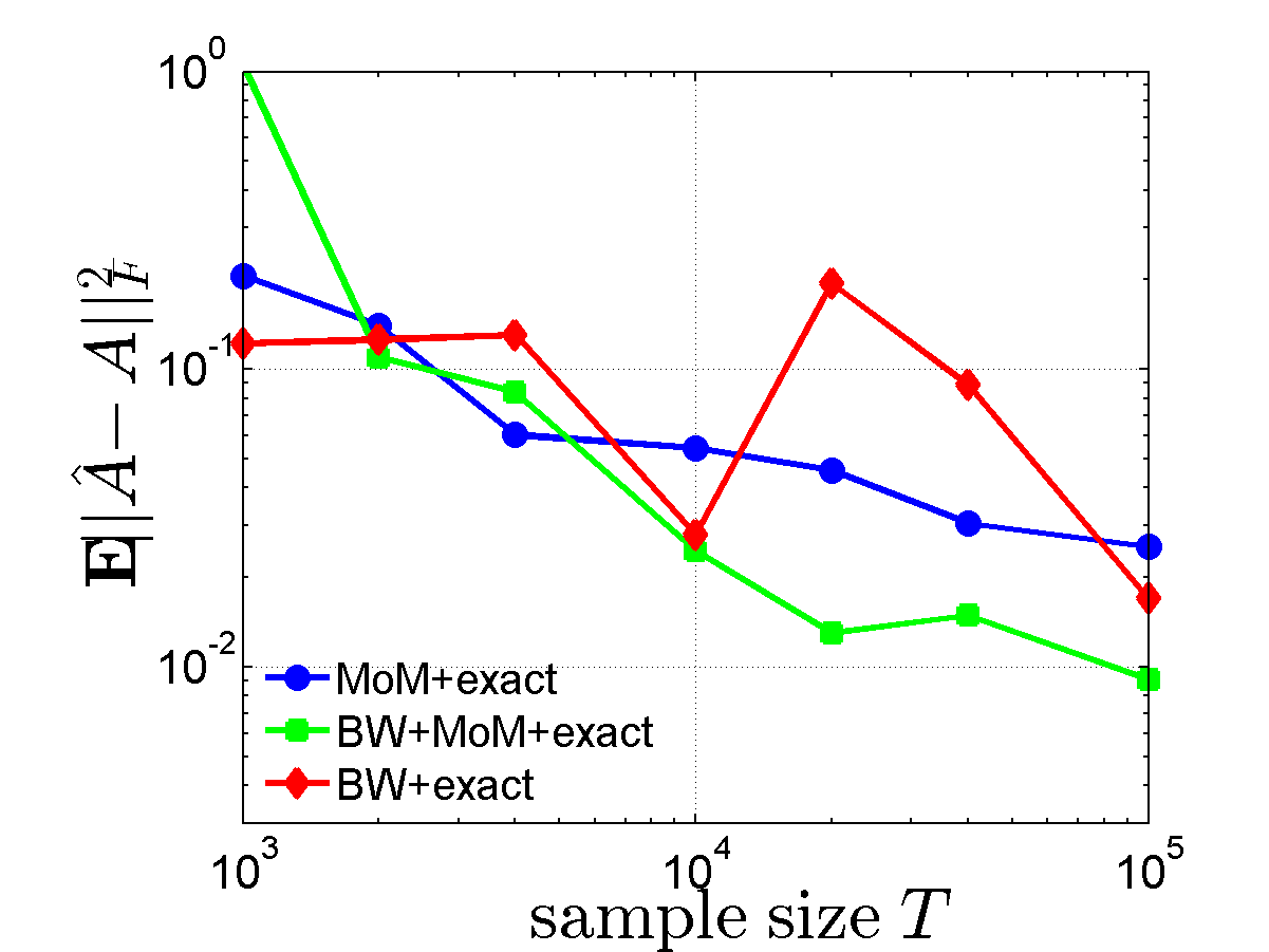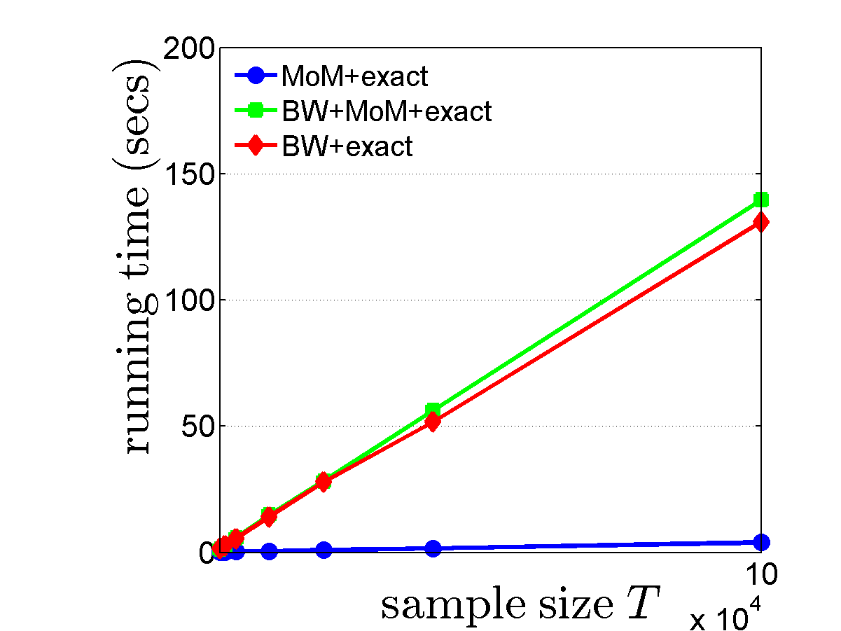
Figure 1. Average error $\mathbb{E}\lVert \hat A - A\rVert^2_{\operatorname{F}}$ and runtime comparison of different algorithms vs. sample size $T$.
Hidden Markov Models (HMM) are a standard tool in the modeling and analysis of time series with a wide variety of applications (see for example Cappé et. al. 2009). Here we consider the problem of learning parametric-output HMMs, where the output from each hidden state follows a parametric distribution from a known family (for example Gaussian, exponential).
We look at discrete-time discrete-space HMMs with $n$ hidden states. The two key parameters governing the HMM are the transition matrix $A$ and the emission law parameters $\boldsymbol \theta$. When the number of hidden states is known, the standard method for estimating the HMM parameters from observed data is the Baum-Welch (BW) algorithm (Baum et al. 1970). This algorithm is known to suffer from two serious drawbacks: (1) it tends to converge very slowly; and (2) it requires a good initial guess as convergence is guaranteed only to a local maximum.
We propose a novel approach to learning parametric-output HMMs, based on the following two insights: (i) in an ergodic HMM, the stationary output distribution is a mixture of distributions from the parametric family, and (ii) given the output parameters, or their approximate values, one can recover in a computationally efficient way the corresponding transition probabilities, up to small additive errors. Combining these two insights leads to our proposed decoupling approach to learning parametric-output HMMs. Rather than attempting, as in the Baum-Welch algorithm, to jointly estimate both the transition probabilities and the output distribution parameters, we instead learn each of them separately.
A code implementing the proposed methods is given in Matlab. For more details see Kontorovich et. al. (2013) and Weiss & Nadler (2015).
Consider a discrete-time HMM with $n$ hidden states $\{1,\dots,n\}$, whose output alphabet $\mathcal{Y}$ is either discrete or continuous. Let $$\mathcal{F}_{\theta} = \{f_{\theta}:\mathcal{Y}\to\mathbb{R} | \theta\in\Theta\}$$ be a family of parametric probability density functions where $\Theta$ is a suitable parameter space. A parametric-output HMM is defined by a tuple \( H = (A,\boldsymbol\theta,\boldsymbol\pi^0) \) where \(A\) is the \(n\times n\) transition matrix between the hidden states \[ A_{ij} = \Pr(X_{t+1} = i | X_{t} = j), \] \(\boldsymbol\pi^0\in\mathbb{R}^n\) is the distribution of the initial state, and the vector of parameters $$\boldsymbol\theta = (\theta_1,\theta_2,\dots,\theta_n)\in\Theta^n$$ determines the $n$ probability density functions $(f_{\theta_1},f_{\theta_2},\dots,f_{\theta_n})$.
To produce the HMM's output sequence, first a Markov sequence of hidden states $X=(X_t)_{t=0}^{T-1}$ is generated via \[ P(X) = \pi_{X_0}\prod_{t=1}^{T-1} P(X_t | X_{t-1}) . \] Next, the output sequence $Y=(Y_t)_{t=0}^{T-1}$ is generated via $$ P(Y | X) = \prod_{t=0}^{T-1} P(Y_t | X_t) = \prod_{t=0}^{T-1} f_{\theta_{X_t}}(Y_t). $$
Learning Problem: Given a long sequence of output symbols $(Y_t)_{t=0}^{T-1}$, estimate the output parameters $\boldsymbol\theta$ and the transition matrix $A$ in a statistically consistent and computationally efficient way.
Assumptions: We make the following standard assumptions:
We first consider the case of a non-aliased HMM, where $\theta_i$ are all distinct, $$\theta_1 \neq \theta_2 \neq \dots \neq \theta_n.$$
We propose the following decoupling approach to learn such an HMM (see Kontorovich et. al. (2013)):
first estimate the output parameters $\boldsymbol \theta = (\theta_1,\theta_2,\dots,\theta_n)$
next estimate the transition probabilities $A$ of the HMM.
Learning the Output Parameters: Assumption 2 implies that the Markov chain over the hidden states is mixing, and so after only a few time steps, the distribution of \(X_t\) is nearly stationary. Assuming for simplicity that already $X_0$ is sampled from the stationary distribution, or alternatively neglecting the first few outputs, this implies that each observable \(Y_t\) is a random realization from the following parametric mixture model , \begin{equation} Y\sim \sum_{i=1}^n \pi_i f_{\theta_i}(y). \label{eq:p_y} \end{equation} Hence, given an output sequence \((Y_t)_{t=0}^{T-1}\), the output parameters \(\theta_i\) and the stationary distribution \(\pi_i\) can be estimated by fitting a mixture model to the observations.
While learning a general mixture is considered a computationally hard problem, recently much progress has been made in the development of efficient methods for learning mixtures under various non-degeneracy conditions, see, e.g., Dasgupta (1999), Achlioptas and McSherry (2005), Moitra and Valiant (2010), Belkin and Sinha (2010), Anandkumar et al. (2012) and references therein.
Learning the Transition Matrix $A$: Next, we describe how to recover the matrix \(A\) given either exact or approximate knowledge of the HMM output distributions.
Define the kernel $K\in\mathbb{R}^{n \times n}$ as the matrix of inner products between the different output distributions: \begin{equation} K_{ij} \equiv \langle f_{\theta_i},f_{\theta_j} \rangle = \int_{\mathcal Y} f_{\theta_i}(y) f_{\theta_j}(y) \text{d}y. \label{eq:K_def} \end{equation} Note that since the HMM is assumed non-aliased, by assumption 1 the kernel matrix $K$ is of full rank $n$.
For many output distribution families, the kernel matrix can be calculated in a closed form. For example, with univariate Gaussian output distributions $\mathcal{N}(\mu,\sigma^2)$, we have that $\theta_i=(\mu_i,\sigma_i^2)$ and the kernel is given by \begin{equation} K_{ij} = \frac{1}{\sqrt{2\pi}} \frac{1}{\sqrt{\sigma_i^2 + \sigma_j^2}} \exp \left( -\frac{1}{2} \frac{(\mu_i - \mu_j)^2}{\sigma_i^2 + \sigma_j^2} \right). \end{equation}
Now, for a consecutive in time observation pair $Y,Y'\in\mathcal{Y}$, define the second order moment matrix $\mathcal{M}\in\mathbb{R}^{n \times n}$ as \begin{equation} \mathcal{M}_{ij} = \mathbb{E}[f_{\theta_i}(Y) f_{\theta_j}(Y')]. \end{equation} Then one can easily show that \begin{equation} \mathcal{M} = K A \operatorname{diag}(\boldsymbol\pi) K^\top. \end{equation}
Thus, given the output sequence \((Y_t)_{t=0}^{T-1}\) and an approximation of $K$ and $\boldsymbol \pi$, we estimate the moment matrix $\mathcal{M}$ by \begin{equation} \hat{\mathcal{M}}_{ij} = \frac{1}{T-1} \sum_{t=0}^{T-2} f_{\theta_i}(Y_t) f_{\theta_j}(Y_{t+1}), \end{equation} and estimate the transition matrix $A$ by solving the following quadratic program: \begin{equation} \label{eq:QPAParam} \hat{A} = \underset{A_{ij} \geq 0,\, \sum_{i}A_{ij}=1}{\arg\!\min} \left \lVert \hat{\mathcal{M}} - (\hat{C}A) \right \rVert_{2}^2, \end{equation} where $\hat{C}_{ij}^{kk'}=\hat{\pi}_j {K}_{kj} {K}_{k' i}$ and $(\hat{C}A)_{kk'}=\sum_{ij} \hat{C}_{ij}^{kk'}A_{ij}$.
As shown in Kontorovich et. al. (2013), this is a consistent estimator (of order $1/\sqrt{T}$) for the transition matrix of the sequence's generating HMM.
Above we assumed that the HMM is non-aliased. For the case of an aliased HMM with two aliased states i,j such that $\theta_i=\theta_j$ see "Learning parametric-output HMMs with two aliased states".
We illustrate our algorithm by some simulation results, executed in MATLAB with the help of the HMM and EM toolboxes (available at www.cs.ubc.ca/~murphyk and www.mathworks.com under "EMGM").
We consider a toy example with $n=4$ hidden states, whose outputs are univariate Gaussians, $\mathcal{N}(\mu_i,\sigma_i^2)$, with $A$ and $\boldsymbol\theta$ given by \begin{equation} A =\left(\begin{array}{cccc} 0.7 & 0.0 & 0.2 & 0.5 \\ 0.2 & 0.6 & 0.2 & 0.0 \\ 0.1 & 0.2 & 0.6 & 0.0 \\ 0.0 & 0.2 & 0.0 & 0.5 \end{array} \right), \quad \begin{array}{rcl} f_{\theta_1} &=& \mathcal{N}(-4,4)\\ f_{\theta_2} &=& \mathcal{N}(0,1)\\ f_{\theta_3} &=& \mathcal{N}(2,36)\\ f_{\theta_4} &=& \mathcal{N}(4,1). \end{array} \end{equation}
To estimate \(A\) we considered the following methods:
method |
initial $\boldsymbol\theta$ |
initial $A$ |
|
|---|---|---|---|
1 |
BW |
random |
random |
2 |
none |
exactly known |
QP |
3 |
none |
EM |
QP |
4 |
BW |
exactly known |
QP |
5 |
BW |
EM |
QP |
6 |
BW |
exactly known |
random |
7 |
BW |
EM |
random |
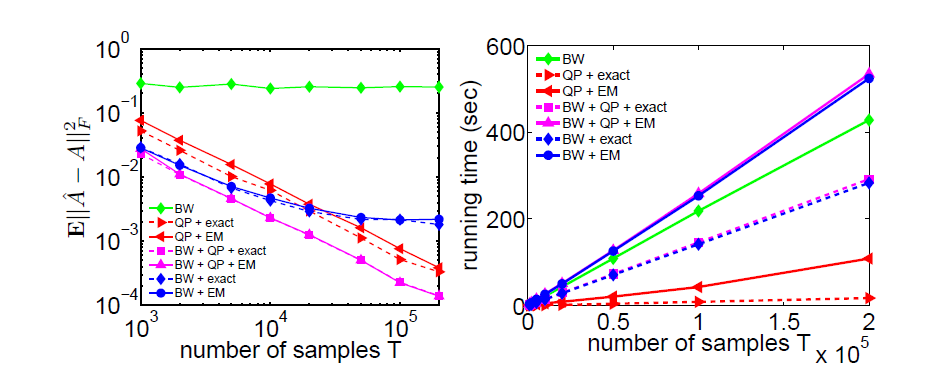
Fig.1 (left) shows on a logarithmic scale $\mathbb{E}\lVert \hat A - A\rVert^2_{\operatorname{F}}$ vs. sample size \(T\), averaged over 100 independent realizations. Fig.1 (right) shows the running time as a function of \(T\). In these two figures, the number of iterations of the BW step was set to 20.
Figure 1. Average error $\mathbb{E}\lVert \hat A - A\rVert^2_{\operatorname{F}}$ and runtime comparison of different algorithms vs. sample size $T$.
Fig.2 (left) shows the convergence of $\mathbb{E}\lVert \hat A - A\rVert^2_{\operatorname{F}}$ as a function of the number of BW iterations, with known output parameters, but either with or without the QP results. Fig.2 (right) gives $\mathbb{E}\lVert \hat A - A\rVert^2_{\operatorname{F}}$ as a function of the number of BW iterations for both known and EM-estimated output parameters with $10^5$ samples.
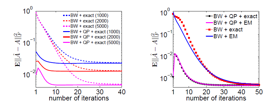
Figure 2. Convergence of the BW iterations.
The simulation results highlight the following points:
These results show the (well-known) importance of initializing the BW algorithm with sufficiently accurate starting values. Our QP approach provides such an initial value for \(A\) by a computationally fast algorithm.
A zip file containing the Matlab implementation code of our estimation procedure can be found here.
In the zip file you will find the following files (among others):
estimateOutputParametersGHMM.m:
Applies the EM algorithm to estimate the Gaussian mixture.
input: data (the sequence) and NumComp (the number of components in the mixture)
output: mu (the estimated Gaussian means), sigma (Gaussian variances) and compWeights (mixture weights)
estimateTransitionMatrixGHMM.m:
Applies a quadradic program to estimate transition matrix $A$.
input: data (the sequence), mu (the Gaussian means), sigma (the Gaussian variances) and compWeights (the mixture weights)
output: the estimated transition matrix $A$
estimateGHMM.m:
Combines the above methods to estimate an HMM
input: data (the sequence) and NumStates (the number of hidden states in the HMM)
output: an estimated HMM (as an instance of the class "AliasGHMM", see below)
estimateGHMM_demo.m: Constructs an HMM, generates data from it and estimate a new HMM from the generated data.
We also provide code for reproducing our simulation results, given in Kontorovich et. al. (2013).
The main file "AliasGHMM.m" consists of the class definition of a HMM with univariate Gaussian output distributions that can have at most two aliased states (see Learning 2-aliased HMMs). Here we only use it for the non-aliased HMM case.
The file "ExpRunSim.m" runs a script that generates an output sequence from the HMM, estimates its parameters according to the proposed procedure and generates graphs for the error in $\hat{A}$ (w.r.t $A$) and the runtimes, for several algorithms.
After the first run, one should get graphs similar to the following: