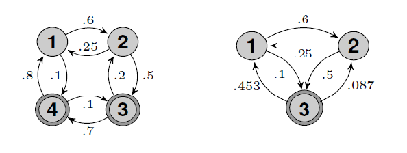
Figure 1. - The aliased HMM (left) and its corresponding non-aliased version with states $3$ and $4$ merged (right).
In a previous page we described our decoupling approach for learning parametric-output HMMs. These results, and the recently proposed spectral and tensor methods for learning HMMs (Hsu et. al. (2012), Anandkumar et. al. (2012)), strongly depend on the assumption that the HMM is non-aliased (namely, all states have different output distributions). In several applications, however, the HMM is aliased, with some states having identical output distributions.
Examples of aliased HMMs include modeling of ion channel gating (Fredkin and Rice (1992)), problems in reinforcement learning (Chrisman (1992), McCallum (1995), Brafman & Shani (2004), Shani et al. (2005)), robot navigation (Jefferies and Yeap (2008), Zatuchna and Bagnall (2009)) and HMMs with several silent states that do not emit any output (Leggetter & Woodland (1994), Stanke and Waack (2003), Brejova et al. (2007)).
The computational efficient learnability of aliased HMMs has been a long standing problem, with only partial solutions provided thus far, see Weiss & Nadler (2015) for discussion. Extending the results in Learning parametric-output HMMs, we here present a method to detect the presence of aliasing and estimate the parameters of a parametric-output HMM with at most 2 aliased states, denoted as 2A-HMM.
A code implementing the proposed methods is given in Matlab. For more details see Weiss & Nadler (2015).
Recall the definition of a parametric-output HMM, $H=(A,\boldsymbol\theta,\boldsymbol{\pi}^0)$, as given in "Learning parametric-output HMMs". For an HMM with output parameters $\boldsymbol \theta=(\theta_1,\theta_2,\dots,\theta_{n})\in\Theta^n$ we say that states $i$ and $j$ are aliased if $\theta_i = \theta_j$. For a 2A-HMM, without loss of generality, we assume that the two aliased states are the two last ones, $n-1$ and $n$. Thus, the parameters of the output distributions for a 2A-HMM satisfy \begin{equation} \theta_1 \neq \theta_2 \neq \dots \neq \theta_{n-1} \qquad \text{and} \qquad \theta_{n-1} = \theta_n. \end{equation} We denote the vector of the $n-1$ unique output parameters of $H$ by \[ \bar{\boldsymbol \theta} = (\theta_1,\theta_2,\dots,\theta_{n-2},\theta_{n-1}) \in \Theta^{n-1}. \] Similarly to the non-aliased case, we define the aliased kernel $\bar K\in\mathbb{R}^{(n-1)\times (n-1)}$ as the matrix of inner products between the $n-1$ different \(f_{\theta_i}\)'s, \begin{equation} \label{eq:K_def_alias} \bar K_{ij} \equiv \langle f_{\theta_i},f_{\theta_j} \rangle \quad i,j\in[n-1] . \end{equation}
In contrast to non-aliased parametric-output HMMs, aliased HMMs are in general not minimal and identifiabale. For a detailed discussion on the minimality and identifiability of 2A-HMMs see Weiss & Nadler (2015). In the following, we assume that the generating HMM is minimal and identifiable.
Recall that $\boldsymbol\pi\in\mathbb{R}^n$ is the stationary distribution over the hidden states and define $\beta= \frac{\pi_{n-1}}{\pi_{n-1} + \pi_{n}}$. We shall make extensive use of the following two matrices, \begin{equation} D = \left( \begin{array}{ccc|cc} & & & 0 & 0 \\[-5pt] & I_{n-2} & & \vdots & \vdots \\ & & & 0 & 0\\ \hline 0 & \dots & 0 & 1 & 1 \\ \end{array} \right) \in \mathbb{R}^{(n-1) \times n} ,\quad C_\beta = \left( \begin{array}{ccc|c} & & & 0 \\[-5pt] & I_{n-2} & & \vdots \\ & & & 0 \\ \hline 0 & \dots & 0 & \beta \\ 0 & \dots & 0 & 1-\beta \\ \end{array} \right) \in \mathbb{R}^{n \times (n-1)}, \end{equation} and the two vectors \begin{equation} {\boldsymbol c_\beta}^{\top} = (0, \dots, 0, {1- \beta}, -\beta)\in\mathbb{R}^n \quad \text{and} \quad \boldsymbol d = (0,\dots, 0,1,-1)^{\top} \in\mathbb{R}^n. \end{equation} These can be viewed as projection and lifting operators, mapping between non-aliased and aliased quantities.
One can show that the transition matrix $A$ of a 2A-HMM can be decomposed as \begin{equation} \label{eq:A-exp} A = C_\beta \bar{A} D + C_\beta \boldsymbol \delta^{\operatorname{out}} \boldsymbol c_\beta^\top + \boldsymbol d (\boldsymbol \delta^{\operatorname{in}})^{\top} D + \kappa\, \boldsymbol d \boldsymbol c_\beta^\top , \end{equation} where \( \bar{A} = D A C_\beta \), \( \delta^{\operatorname{out}} = D A \boldsymbol d \), \( \delta^{\operatorname{in}} = \boldsymbol c_\beta^\top A C_\beta \) and \( \kappa = \boldsymbol c_\beta^\top A \boldsymbol d \).
As shown below, this decomposition will be convenient for recovering the transition matrix entries from the observed data.
In this section we study the problems of detecting whether the HMM is aliasing and recovering its transition matrix $A$, all in terms of $(Y_t)_{t=0}^{T-1}$. We assume the HMM is either non-aliasing, with $n-1$ states, or 2-aliasing with $n$ states.
The proposed learning procedure consists of the following steps:
Estimate the $n-1$ unique output distribution parameters $\bar{\boldsymbol{\theta}}$ and the projected stationary distribution $\bar{\boldsymbol{\pi}}$ by fitting a mixture as in the non-aliased case.
In case of a non-aliased HMM, estimate the $(n-1)\times(n-1)$ transition matrix $\bar A$, as in the non-aliased case.
In case of a 2-aliased HMM, identify the component $\theta_{n-1}$ corresponding to the two aliased states, and estimate the $n\times n$ transition matrix $A$.
For methods to solve steps (i) and (iii), see Learning non-aliased HMMs. We now describe in more detail steps (ii) and (iv).
Moments: To solve problems (ii) and (iv), we first introduce the moment-based quantities we shall make use of. Given $\bar{\boldsymbol \theta}$ and $\bar{\boldsymbol \pi}$ or estimates of them, for any $i,j\in[n-1]$, we define the second order moments with time lag $t$ by \begin{equation} \label{eq:mom-def} \mathcal{M}^{(t)}_{ij} = \mathbb{E}[f_{\theta_i}(Y_0) f_{\theta_j}(Y_{t})] ,\quad t\in\{1,2,3\}. \end{equation} The consecutive in time third order moments are defined by \begin{equation} \label{eq:momT-def} \mathcal{G}^{(c)}_{ij} = \mathbb{E}[f_{\theta_i}(Y_0) f_{\theta_c}(Y_{1}) f_{\theta_j}(Y_{2})] ,\quad \forall c\in[n-1]. \end{equation} We also define the lifted kernel, $\mathcal{K} = D^{\top} \bar{K} D \in \mathbb{R}^{n\times n}$.
One can verify that for a 2A-HMM, \begin{align} \label{eq:mom-2A} \mathcal{M}^{(t)} & = \bar{K} D A^{t} C_\beta \operatorname{diag}(\bar{\boldsymbol \pi}) \bar{K}\\ \mathcal{G}^{(c)} & = \bar{K} D A \operatorname{diag}( {\mathcal{K}}_{[\cdot,c]}) A C_\beta \operatorname{diag}(\bar{\boldsymbol \pi}) \bar{K}. \end{align} Next we define the kernel free moments $M^{(t)},G^{(c)}\in\mathbb{R}^{(n-1)\times(n-1)}$ as follows: \begin{align} \label{eq:striped-mom} M^{(t)} &= \bar{K}^{-1} \mathcal{M}^{(t)} \bar{K}^{-1} \operatorname{diag}(\bar{\boldsymbol \pi})^{-1} \\ \label{eq:striped-momT} G^{(c)} & = \bar{K}^{-1} \mathcal{G}^{(c)} \bar{K}^{-1} \operatorname{diag}(\bar{\boldsymbol \pi})^{-1}. \end{align}
Let $R^{(2)},R^{(3)},F^{(c)}\in\mathbb{R}^{(n-1)\times (n-1)}$ be given by \begin{align} \label{eq:deltaM2} R^{(2)} &= M^{(2)} - (M^{(1)})^2\\ \label{eq:deltaM3} R^{(3)} &= M^{(3)} - M^{(2)} M^{(1)} - M^{(1)} M^{(2)} + (M^{(1)})^3 \\ \label{eq:deltaGk} F^{(c)} &= G^{(c)} - M^{(1)} \operatorname{diag}(\bar{K}_{[\cdot,c]}) M^{(1)}. \end{align} We have the following key relations between these moments and the decomposition of the transition matrix $A$ (assuming w.l.g that the aliased component is $\theta_{n-1}$): \begin{align} \label{eq:momtoA1} M^{(1)} & = \bar{A} \\ \label{eq:dmomtoA2} R^{(2)} & = \boldsymbol{\delta}^{\operatorname{out}} (\boldsymbol{\delta}^{\operatorname{in}})^\top \\ \label{eq:dmomtoA3} R^{(3)} & = \kappa R^{(2)} \\ \label{eq:dmomTtoA} F^{(c)} & = \bar{K}_{{n-1},c} R^{(2)} ,\quad \forall c\in[n-1]. \end{align}
We now use these relations to detect aliasing, identify the aliased states, and recover the aliased transition matrix $A$.
Detection of aliasing: It can be shown that a HMM is aliasing if and only if $R^{(2)}\neq0$. Thus, motivated by Kritchman & Nadler (2009), we adopt the largest singular value $\hat\sigma_1$ of $R^{(2)}$ as our test statistic. The resulting test is \begin{equation} \text{if } \hat\sigma_1\geq h_T \text{ return "2-aliased"}, \text{ otherwise return "non-aliased"}, \end{equation} where $h_T = \Omega(T^{-\frac{1}{2}+ \varepsilon})$ is a predefined threshold with $0<\varepsilon<\frac{1}{2}$.
Indetifying the aliased states: From the fourth relation above, we estimate the index $i\in[n-1]$ of the aliased component by solving the following least squares problem: \begin{equation} \label{eq:acestimate} \hat i = \operatorname{argmin}_{i\in[n-1]} \sum_{c\in [n-1]} \lVert \hat{F}^{(c)} - \bar{K}_{i,c} \hat{R}^{(2)} \rVert_{\operatorname{F}}^2. \end{equation}
Estimating the aliased transition matrix $A$: Given the aliased component, we estimate the $n\times n$ transition matrix $A$ by using the form of its decomposition. Since $R^{(2)}$ is rank $1$, we write its singular value decomposition as $R^{(2)} = \sigma \boldsymbol{u} \boldsymbol{v}$. As singular vectors are determined only up to scaling, we have that \begin{equation} \boldsymbol{\delta}^{\operatorname{out}} = \gamma \boldsymbol u \qquad \text{and} \qquad \boldsymbol{\delta}^{\operatorname{in}} = \frac{\sigma}{\gamma} \boldsymbol v, \end{equation} where $\gamma\in\mathbb{R}$ is a yet undetermined constant. Thus, the decomposition of $A$ takes the form: \begin{equation} \label{eq:A-exp-bg} A = C_{\beta} \bar{A} D + \gamma C_{\beta} \boldsymbol u \boldsymbol{c}_{\beta}^\top + \frac{\sigma}{\gamma} \boldsymbol{d} \boldsymbol{v}^{\top} D + \kappa\, \boldsymbol{d} \boldsymbol{c}_{\beta}^\top . \end{equation} Since $\bar{A}, \sigma, \boldsymbol u$, and $\boldsymbol v$ were estimated in previous steps, we are left to determine the scalars $\gamma$, $\beta$, and $\kappa$ .
As for $\kappa$, we have $R^{(3)} = \kappa R^{(2)}$. Thus, plugging the empirical versions, $\hat \kappa$ is estimated by \begin{equation} \label{eq:dmomoest} \hat \kappa = \operatorname{argmin}_{r\in\mathbb{R}} \lVert \hat{R}^{(3)} - r \hat{R}^{(2)}\rVert_{\operatorname{F}}^2. \end{equation}
Finally, in order to estimate $\gamma$ and $\beta$ define the objective function $h:\mathbb{R}^2\to\mathbb{R}$ by \begin{equation} h(\gamma',\beta') = \min_{i,j\in[n]} \{\gamma' A'_H(\gamma',\beta')_{ij} \}, \end{equation} where \begin{equation} A'_H(\gamma',\beta') \equiv C_{\beta'} \bar{A} D + \gamma' C_{\beta'} \boldsymbol u {\boldsymbol{c}_{\beta'}}^\top + \frac{\sigma}{\gamma'} \boldsymbol{d} \boldsymbol{v}^{\top} D + \kappa\, \boldsymbol{d} {\boldsymbol{c}_{\beta'}}^\top. \end{equation} Assuming that the HMM is identifiable, it is shown in Weiss & Nadler (2015) that $\gamma'=\gamma$ and $\beta'=\beta$ is the unique solution of \begin{equation} \label{eq:opt} (\hat \gamma,\hat \beta) = \operatorname{argmax}_{(\gamma',\beta')\in[0,\frac{2}{\sigma}]\times[0,1]} {h(\gamma',\beta')}. \end{equation} This two-dimensional optimization problem can be solved by either brute force or any non-linear problem solver.
Having an estimate for all the parameters in the decomposition, the above procedure provides an estimate for the aliased transition matrix $A$. It is shown in Weiss & Nadler (2015) that this method is consistent.
The following simulation results illustrate the consistency of our methods to detect aliasing, identify the aliased component, and learn the transition matrix $A$. As our focus is on the aliasing, we assume for simplicity that the output parameters $\bar{\boldsymbol{\theta}}$ and the projected stationary distributions $\bar{\boldsymbol{\pi}}$ are exactly known.
We consider the following HMM $H$ with $n=4$ hidden states, see Figure 1 (left). The output distributions are univariate Gaussians $\mathcal{N}(\mu_i,\sigma_i^2)$, the matrix $A$ and $(f_{\theta_i})_{i=1}^4$ are given by \begin{equation} A =\left(\begin{array}{cccc} 0.3 & 0.25 & 0.0 & 0.8 \\ 0.6 & 0.25 & 0.2 & 0.0 \\ 0.0 & 0.5 & 0.1 & 0.1 \\ 0.1 & 0.0 & 0.7 & 0.1 \end{array} \right), \quad \begin{array}{rcl} f_{\theta_1} &=& \mathcal{N}(3,1)\\ f_{\theta_2} &=& \mathcal{N}(6,1)\\ f_{\theta_3} &=& \mathcal{N}(0,1)\\ f_{\theta_4} &=& \mathcal{N}(0,1). \end{array} \end{equation} States $3$ and $4$ are aliased and this 2A-HMM is identifiable. The rank-1 matrix $R^{(2)}$ has a singular value $\sigma=0.33$. Figure 1 (right), shows its non-aliased version, $\bar{H}$, with states $3$ and $4$ merged.
Figure 1. - The aliased HMM (left) and its corresponding non-aliased version with states $3$ and $4$ merged (right).
To test our aliasing detection algorithm, we generated $T$ outputs from the original aliased HMM and from its non-aliased version $\bar{H}$.
Fig.2 (top left) shows the empirical densities (averaged over $1000$ independent runs) of the largest singular value of $\hat{R}^{(2)}$, for both $H$ and $\bar{H}$.
Fig.2 (top right) shows similar results for a 2A-HMM with $\sigma=0.22$.
When $\sigma=0.33$, already $T=1000$ outputs suffice for essentially perfect detection of aliasing. For the smaller $\sigma=0.22$, more samples are required.
Fig.2 (middle left) shows the false alarm and misdetection probabilities vs. sample size \(T\) of the aliasing detection test with threshold $h_T=2T^{-\frac{1}{3}}$. The consistency of our method is evident.
Fig.2 (middle right) shows the probability of misidentifying the aliased component $\theta_{\bar 3}$. We considered the same 2A-HMM $H$ but with different means for the Gaussian output distribution of the aliased states, $\mu_{{\bar 3}} = \{0,1,2\}$. As expected, when $f_{\theta_{\bar 3}}$ is closer to the output distribution of the non-aliased state $f_{\theta_1}$ (with mean $\mu_1=3$), identifying the aliased component is more difficult.
Finally, we considered the following methods to estimate \(A\):
The Baum-Welch algorithm with random initial guess of the HMM parameters (BW)
Our method of moments with exactly known \(\bar{\boldsymbol \theta}\) (MoM+Exact)
BW initialized with the output of our method (BW+MoM+Exact)
BW with exactly known output distributions but random initial guess of the transition matrix (BW+Exact)
Fig.2 (bottom left) shows on a logarithmic scale the mean square error $\mathbb{E}\lVert\hat A - A\rVert_{\operatorname{F}}^2$ vs. sample size $T$, averaged over 100 independent realizations. Fig.2 (bottom right) shows the running time as a function of $T$. In both figures, the number of iterations of the BW was set to 20.
These results show that with a random initial guess of the HMM parameters, BW requires far more than 20 iterations to converge. Even with exact knowledge of the output distributions but a random initial guess of the matrix \(A\), BW still fails to converge after 20 iterations. In contrast, our method yields a relatively accurate estimator in only a fraction of run-time. Furthermore, using this estimator as an initial guess for BW yields even better accuracy.
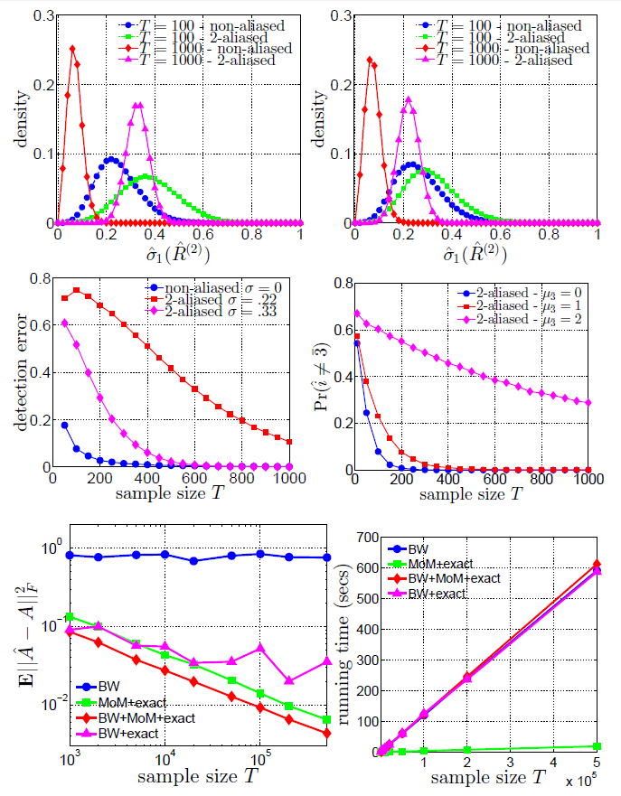
Figure 2. - Top: Empirical density of the largest singular value of $R^{(2)}$ with $\sigma=0.33$ (left) and $\sigma=0.22$ (right). Middle: Misdetection probability of aliasing/non-aliasing (left) and probability of misidentifying the correct aliased component (right). Bottom: Average error $\mathbb{E}\lVert \hat A - A\rVert^2_{\operatorname{F}}$ and runtime comparison of different algorithms vs. sample size $T$.
A Matlab implementation of our estimation procedure can be found here.
The main file "AliasGHMM.m" is the class definition of a HMM with univariate Gaussian output distributions that can have at most two aliased states. This class consists all the methods needed for defining an aliased Gaussian HMM, genereting samples from it and all methods needed for the estimation of a 2-aliased HMM from a given output sequence.
The file "ExpRunAliasSim.m" runs a script that generates an output sequence from the aliased HMM in Section 5, estimates its parameters by the proposed procedure and generates graphs for the error in $\hat{A}$ (w.r.t $A$) and the runtimes for several algorithms.