Estimating the accuracies of multiple classiﬁers without labeled data

Unsupervised Ensemble Learning

Written by Ariel Jaffe and Boaz Nadler, 2015

Introduction
Problem Setup
Spectral Methods for Binary Ensembles
Code
References

1. Introduction

Consider for simplicity a binary classification problem, for which we are given $m$ pre-constructed classifiers, $f_1,\ldots,f_m$. The main task in ensemble learning is to construct a more accurate meta learner from this group of $m$ possibly weak learners.
There are two main ensemble learning scenarios:

Supervised ensemble learning: The inputs are a labeled validation set, consisting of pairs of instances and their corresponding labels, $(x_j,y_j)$, as well as the predictions of the $m$ classifiers, $f_i(x_j)$. In this scenario the accuracy of the various classifiers can be estimated since we have true labels.
Numerous algorithms have been proposed for training a meta classifier in this setup, see [3] , [4] and references therein.
Unsupervised ensemble learning: In this scenario, the input is a (potentially large) unlabeled set of instances $x_j$, and the predictions of the $m$ classifiers, $f_i(x_j)$. The key point, that makes this setup challenging, is that we have no labeled data at all.
This creates a problem - without labeled data, we cannot directly assess the accuracy of the $m$ classifiers, as in the previous setup. It is thus not clear how can we construct a more accurate meta classifier.
In this page, we describe a spectral approach and corresponding code, to handle this unsupervised setup in the specific case of binary classification, under certain assumptions detailed below. For more details see [1] and [2].

2. Problem Setup

Consider an ensemble of $m$ binary classifiers, all operating on the same instance space $\mathcal X$ (typically $\mathbb{R}^d$), with an output space $\mathcal Y = \{1,-1\}$. Since the classifiers are binary, they are fully defined by their sensitivity and specificity, denoted $\psi$ and $\eta$ respectively:
$$ \psi_i = \Pr[f_i(X)=1|y=1] \quad \eta_i = \Pr[f_i(X)=-1|y=-1] $$ Given only the $m\times n$ matrix $Z$ of classifiers predictions, where $Z_{ij}=f_i(x_j)$ can one:

Estimate the accuracies of the different classifiers?
Combine the classifiers to an improved meta classifier?

Dawid and Skene [5] were among the first to study this setup, and propose an expectation maximization (EM) algorithm, to estimate the unknown specificities and sensitivities of all $m$ classifiers and the labels $y_j$ of the $n$ instances. In recent years, with the popularity of crowdsourcing, several works studied similar scenarios, and also suggested EM based approaches, see for example [6] ,[7] ,[8] and [9].

The key assumption made by Dawid and Skene, which we also adopt in our work is that of conditionally independent classifiers. Namely, that conditional on the class label, different classifiers make independent predictions. That is, for all $f_i,f_j$ and for all labels $a_i,a_j \in \{-1,1\}$, $$ \Pr[f_i(x)=a_i,f_j(x)=a_j\,|y] = \Pr[f_i(x)=a_i|y] \cdot \Pr[f_j(x)=a_j\,|y] $$ In fact, assuming all classifiers are conditionally independent (and not only in pairs, as in the above equation), our problem is equivalent to learning a mixture of discrete (binary) product distributions, see [10]. In recent years several works have used the low rank structure of the second and third moments of the data in order to estimate the parameters of the mixture, see [11] and [12].

3. Spectral Methods for Binary Ensembles

In our work, we build upon the spectral approach developed in [2] , which is based on a study of the $m\times m$ covariance matrix of the $m$ classifiers.

An important lemma, presented in [2] is the rank-1 structure of the off-diagonal elements of this matrix: $$ r_{ij} = (1-b^2)(\psi_i+\eta_i-1) (\psi_j+\eta_j-1),$$ where $b=\Pr(Y=1)-\Pr(Y=-1)$ denotes the class imbalance.
Furthermore, as shown in [1], the population mean of the $i$-th classifier is given by $$ \mu_i = (\psi_i-\eta_i) + b (\psi_i+\eta_i-1).$$ When the class imbalance is apriori known, using the above two quantities, it is easy to estimate the unknonw parameters $\psi_i,\eta_i$ of the $m$ classifiers (see Section 3 in [1]).

When $b$ is unkown, we propose the following two methods to estimate it, and then estimate $\psi_i,\eta_i$ using $\hat b$.

The first is based on the joint covariance tensor, $T_{ijk} = \mathbb E[(f_i-\mu_i)(f_j-\mu_j)(f_k-\mu_k)]$, whose off diagonal elements correspond to a rank-1 tensor: $$ T_{ijk}= -b(1-b^2)(\psi_i+\eta_i-1) (\psi_j+\eta_j-1)(\psi_k+\eta_k-1)$$ Note that the vectors constructing $r_{ij}$ and $T_{ijk}$ are both proportional to $(\psi_i+\eta_i-1)$. In [1] , we use this observation to construct an estimate for $b$. We refer to this method as the 'tensor method'.
The second approach to estimate $b$ is based on the log-likelihood of our data: $$ \log\bigg( \prod_{j=1}^n \Pr(Z_{1j}, \ldots, Z_{mj}\bigg) = \sum_{j=1}^n \log\Pr(Z_{1j}, \ldots, Z_{mj})$$ Note that the likelihood is a function of $2m+1$ variables: $\{\psi_i\}_{i=1}^m$,$\{\eta_i\}_{i=1}^m$ and $b$. However, every guess for $b$ yields corresponding guesses for the remaining variables. We can therefore scan over $b \in [-1+\delta, 1-\delta]$, where $\delta>0$ corresponds to an a-priori bound on the class imbalance, and find the value which maximizes the log likelihood function. We denote this as the 'restricted likelihood' method.

4. Code

A matlab implementation of our unsupervised methods can be found here.
The file contains the following functions:

function b_hat = estimate_class_imbalance_tensor(Z,delta)

Input:
Z - $m \times n$ matrix containing the binary ($-1$ or $1$) predictions of $m$ classifiers over $n$ independent instances.
delta - the class imbalance estimation will be bounded away from $-1$ and $1$ by $\delta$.
Output:
b_hat - the estimate for the class imbalance by the tensor approach.
b_hat = estimate_class_imbalance_restricted_likelihood(Z,delta)

Similar to the previous function, except that the estimate is done by the restricted likelihood approach.
[V_hat,psi_hat,eta_hat] = estimate_ensemble_parameters(Z,b)

Input:
Z - $m \times n$ prediction matrix.
b - class imbalance (exact or estimated).
Output:
V_hat - first eigenvector of the covariance matrix $R$.
psi_hat - $m \times 1$ vector of estimated sensitivities.
eta_hat - $m \times 1$ vector of estimated specificities.

Additional routines (some required by the procedures above):

function [y,Z] = generate_prediction_matrix(m,n,b,psi,eta) - generates a random vector of true lablels y, and a random prediction matrix $Z$.

function R = estimate_rank_1_matrix(Q) - receives a $m \times m$ matrix and estimates its diagonal values, by assuming that the matrix is (or close to) rank 1.

function T = compute_classifier_3D_tensor(Z) - receives the prediction matrix $Z$ and returns the sample covariance tensor.

function alpha = estimate_alpha(V,T) - estimates the value of $\alpha(b)$, used by the tensor method to estimate $b$.

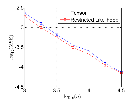
We also provide a demo code which generates synthetic random data and reproduces the following figure from [1] . This figure shows the mean square error $\mathbb{E}[(\hat b-b)^2]$ in estimating the class imbalance, vs. the number of instances over a log-log scale, of the two methods described above. As seen from the figure, on simulated data the restricted likelihood approach is more accurate than the tensor-based one.

5. References

A. Jaffe, B. Nadler, Y. Kluger, Estimating the accuracies of multiple classifiers without labeled data , AISTATS-2015.
F. Parisi, F. Strino, B. Nadler, Y. Kluger, Ranking and Combining Multiple predictors without labeled data Proceedings of the National Academy of Sciences, vol. 111(4), 1253-1258, 2014.
L. I. Kuncheva, Combining pattern classifiers: methods and algorithms. John Wiley & Sons, 2004.
T. G. Dietterich, Ensemble Methods in Machine Learning. Multiple classifier systems. Springer Berlin Heidelberg, 2000. 1-15.
A. P. Dawid and A. M. Skene, Maximum likelihood estimation of observer error-rates using the EM algorith. Journal of the Royal Statistical Society, 1979.
V.C. Raykar, Y. Shipeng, L.H. Zhao, G.H. Valdez, C. Florin, L. Bogoni, and Moy L, Learning from crowds. Journal of Machine Learning Research, 2010.
J. Whitehill, P. Ruvolo, T. Wu, J Bergsma, and J.R. Movellan, Whose vote should count more: Optimal integration of labels from labelers of unknown expertise. In Advances in Neural Information Processing Systems 22, 2009.
P. Welinder, S. Branson, S. Belongie, and P. Perona, The multidimensional wisdom of crowds. In Advances in Neural Information Processing Systems 23, 2010.
P. Donmez, G. Lebanon, and K. Balasubramanian, Unsupervised Supervised Learning I: Estimating Classification and Regression Errors without Labels. The Journal of Machine Learning Research 11 (2010).
Y. Freund and Y. Mansour, Estimating a mixture of two product distributions. In Proceedings of the 12th Annual Conference on Computational Learning Theory,1999.
A. Anandkumar, D. Hsu, and S.M. Kakade, A method of moments for mixture models and hidden Markov models. In Conference on Learning Theory, 2012.
Y. Zhang, X. Chen, D. Zhou, and M.I. Jordan, Spectral methods meet EM: A provably optimal algorithm for crowdsourcing. In Advances in Neural Information Processing Systems 27, 2014.